Using a Variational Auto-encoder to predict protein function

NEWS: This work was accepted as an oral presentation at NIPS MLCB workshop. See the extended abstract.

In this post I report an application of a Variational Auto-Encoder to predict the effects of mutations on protein function. This post can serve as an “open notebook” for interested machine learning researchers to suggest improvements. If you think you have good ideas upon reading this, do not hesitate to contact me (you can find my contact information at the footer of this page).

Big Picture

Proteins are responsible for the most diverse set of functions in biology. What proteins do is largely determined by their sequence (and conditions under which they fold). The ability to predict whether a change in sequence will affect their function is extremely valuable. There is a clear engineering/clinical incentive to modify protein function. For instance, my collaborators synthesize massive libraries of AAV variants, hoping to find effective viral vectors for gene therapy.

My interest in this topic, as a computational biologist with interest in origin of life (and evolution), is driven more directly by basic science. Imagine you have a protein of size \(L\). The standard \(20\) amino-acid alphabet that could appear in any from position \(1\) to \(L\). This means that there are \(20^L\) possible sequences of size \(L\). A key question in the field of origin of life, as well as evolutionary theory is this:

How many of these \(20^L\) sequences result in a (specific) function?

In other words, how dense is the sequence space in functional proteins? This space grows exponentially with sequence size, hence it is hopeless to sample it thoroughly even by computational means, let alone experiments. But navigating it in search for a function may also not be as bad as it initially seems, in particular, if functions are concentrated in clusters of (nearby) sequences. We can start from a known sequence that does have that function, and explore its vicinity.

For the readers that are not very familiar with biology, maybe an analogy could be helpful. The English alphabet has 26+1 (for space) letters. For a sentence of length \(L\), there are \(27^L\) possible arrangments of these letters, most of them will have no meaning in English. However, a lot of sentences that do have a meaning are fairly close to each other. Hence, starting from a set of meaningful sentences, we can hope to train a model to reproduce them with some novelty. The problem for the protein engineer is significantly harder, because checking whether your algorithm produced a meaningful sequence requires you to actually make the protein (and deploy it in the right biological context) to evaluate its function. With sentences, verification is significantly easier and cheaper (a human can read and verify it). So the goal is to find a computational method where we can predict whether a sequence is functional (bio-active).

In this blog post, I mention one approach I’ve recently tried with some success to predict protein functionality. I train a Variational Auto-encoder[1] on protein sequences that are close to each other (from an evolutionary perspective) and using that I try to predict how much the function of the protein is affected by changing one or two letters in a sequence. This is of course a much simpler problem than the big picture described above (but a first natural step to it). However, even when the problem is this much simpler, predicting protein function using current methods still has much room for improvement.

Background

A lot of recent success in machine learning, particularly in vision, is indebted to the vast amount of data that are compiled and accessible on the internet. Biologists have also become very good at generating massive amounts of data, especially sequence data from a variety of organisms. As a result, for many sequences of interest (be it DNA or protein sequences), one can search a huge database of sequences that are observed in other organisms, and align them to the sequence of interest (up to an arbitrarily constrained similarity threshold). This is called a multiple sequence alignment (MSA). An MSA constitutes an evolutionary cluster of nearby sequences. Note however, that these large datasets don’t generally come with “labels” (e.g. we don’t have a quantitative idea of how fast each protein metabolizes a compound). But because these sequences are observed in living organisms, we can safely assume that they are functional, and because of their similarity, they likely do similar things. Datasets that do provide quantitative measurements of function exist for some proteins (and we will make use of them, but not for training). But their size (and diversity) is generally more suitable for validation, rather than training. Hence, an unsupervised model seems to be a useful approach for this particular problem.

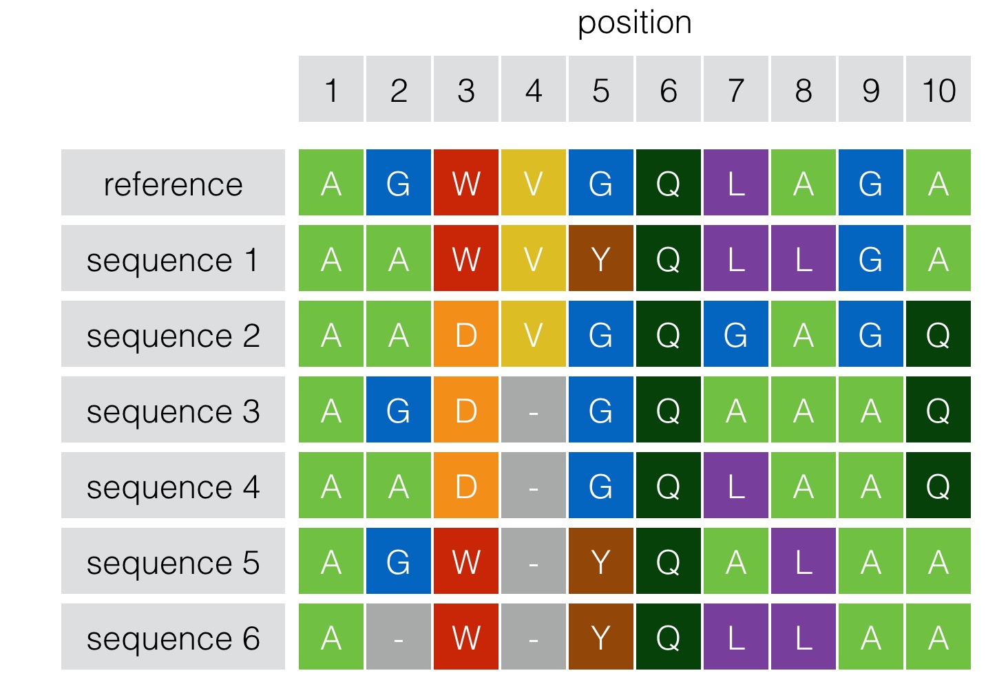
So what can we learn from alignment data? The toy model presented above can serve as an example. The alignment versus the reference sequence for 6 related sequences are shown. We can see for instance that columns (positions) 1 and 6 are fully conserved (independent of others). An “independent” model, learns the distribution of amino-acids in each column, and ascribes probabilities to each sequence accordingly. But there is more to learn from this data. If we start looking at pairwise interactions along the sequence, for instance, it appears that positions 3 and 10 have a pairwise interaction as D is always paired with Q, and W is always paired with A (this would be missed by an independent model). If our model is able to capture even higher order correlations, we can even say that it may be that position 5 also interacts with positions 3 and 10. In biology, mutations don’t necessarily affect the function independently (what is known as epistasis). One mutation alone may be detrimental, but another one at a different position may “rescue” the protein to its original functionality.

Based on this intuition, over the past few years generative models have been used on sequence alignments to predict protein structure and function [1],[2]. These models learn correlations between amino acids in different positions, and then try to guess (approximately) whether a change from one amino-acid to another in a given position(s) would be beneficial or detrimental for the function of the protein. The most successful applications of this approach have used Potts models as their core modeling approach. This approach models independent and pairwise interactions along the sequence. You can read the technical details here and see its application for a large set of datasets here. The methods show that harnessing correlations between pairs of amino acids at different positions provides significant power for protein folding and function prediction.

In this post I show how to use a simple VAE [3] (another generative approximation method), to almost reproduce the results as predicted by the Potts model approach. Using auto-encoders for unsupervised protein fitness prediction has been a subject of interest for many groups. In fact, John Ingraham and Adam Reisselman from Marks lab have presented independently developed results on this at Broad MIA.

Results

I directly use the alignment data that accompanies Hopf, Ingraham, et al’s recent paper in Nature biotechnology and show that a simple VAE can perform closely to the performance of their model (in some cases with fewer parameters) in the single mutation and double mutation case. This method however should be seen as work in progress, as the VAE does not outperform the Potts model approach. The full workflow can be accessed in this notebook. I highlight general results in this blog post.

Before proceeding, I’d like to clarify two bits of terminology. First, in the entire workflow, we have one sequence that anchors our analysis. We run the alignment against that sequence (where we call it reference), and then we look at single, or double mutants of that sequence (these often don’t exists in the alignment, but we have experimental data for their function). In that context, I refer to the reference sequence as the “wildtype”. Second, fitness is a vague biological term. For our purposes, since what is being measured in each dataset may not be exactly the same thing, it is convenient to refer to it as fitness. As our interest is in relative performance (on whatever metric) between mutants, this is not unreasonable.

To calculate a fitness value for particular sequence, I train a VAE with the following architecture on the alignment data:

batch_size = 20
original_dim=len(ORDER_LIST)*PRUNED_SEQ_LENGTH
output_dim=len(ORDER_LIST)*PRUNED_SEQ_LENGTH
latent_dim = 2
intermediate_dim = 250
nb_epoch = 10
epsilon_std = 1.0
#np.random.seed(1337)  # for reproducibility

def sampling(args):
    z_mean, z_log_var = args
    epsilon = K.random_normal(shape=(batch_size, latent_dim), mean=0.,
                              std=epsilon_std)
    return z_mean + K.exp(z_log_var / 2) * epsilon

def vae_loss(x, x_decoded_mean):
    xent_loss = original_dim * objectives.categorical_crossentropy(x,  x_decoded_mean)
    kl_loss = - 0.5 * K.sum(1 + z_log_var - K.square(z_mean) - K.exp(z_log_var), axis=-1)
    return xent_loss + kl_loss

#Encoding Layers
x = Input(batch_shape=(batch_size, original_dim))
h = Dense(intermediate_dim,activation="elu")(x)
h= Dropout(0.7)(h)
h = Dense(intermediate_dim, activation='elu')(h)
h=BatchNormalization(mode=0)(h)
h = Dense(intermediate_dim, activation='elu')(h)

#Latent layers
z_mean=Dense(latent_dim)(h)
z_log_var=Dense(latent_dim)(h)
z = Lambda(sampling, output_shape=(latent_dim,))([z_mean, z_log_var])

#Decoding layers 

decoder_1= Dense(intermediate_dim, activation='elu')
decoder_2=Dense(intermediate_dim, activation='elu')
decoder_2d=Dropout(0.7)
decoder_3=Dense(intermediate_dim, activation='elu')
decoder_out=Dense(output_dim, activation='sigmoid')
x_decoded_mean = decoder_out(decoder_3(decoder_2d(decoder_2(decoder_1(z)))))

vae = Model(x, x_decoded_mean)

#Potentially better results, but requires further hyperparameter tuning
#optimizer=keras.optimizers.SGD(lr=0.005, momentum=0.001, decay=0.0, nesterov=False,clipvalue=0.05)
vae.compile(optimizer="adam", loss=vae_loss,metrics=["categorical_accuracy","fmeasure","top_k_categorical_accuracy"])

The hyperparameters for this model are manually optimized, but when using the ADAM optimizer, the results are generally not radically affected by reducing one or two layers, adding dropout, or adding more regularization. SGD is significantly more sensitive to these manipulations, but it is also thought to be potentially better at finding state of the art results. I have not managed to beat the results obtained by ADAM when using SGD.

Once the network is trained, I use it to predict the probability of a mutant. To do so, I reconstruct the sequence it was fed, using its internal model (this is what an auto-encoder does).

The one-hot encoding (input) of a sequence looks (almost) like this:

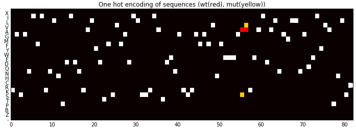
The reason I say almost is, that here I have actually superimposed two one hot encodings from two sequences. One is the wildtype sequence, and the other is the mutant. The white squares are shared between the two sequences. The colors show where the wildtype (red) and the mutant (yellow) differ in sequence, in this case in two positions. The one hot vector for each sequence is what is fed into the network. In the next two panels, I show the reconstruction of the two sequences by the trained network.

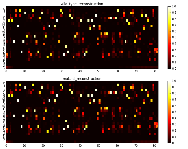
These reconstructions are normalized like a probability weight matrix, where each position column constitutes probabilities for each amino-acid at that location (we denote this matrix as \(P\) below).

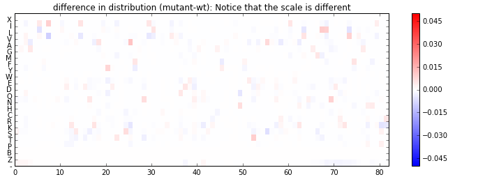
The most interesting take away (and the reason I tried this) from these reconstructions is what the network has learned about co-dependence of mutations. To see this better, I subtract the the two PWMs and look at their difference below. The update in probability occurs not only in the position where the two sequences differ, but also in places that they are the same. The model is suggesting that maybe an additional mutation (for instance a “rescue”) in those places is now more likely (or less likely) given the mutation observed.

Using these reconstructions, I compute the (log) probability of a sequence as:

\[\mathbb{P}(\sigma)=\log(trace(H^T P))\]

Where \(H\) is the one-hot encoding of the sequence of interest, and \(P\) is the probability weight matrix generated by feeding the network a sequence. This formula allows me to calculate how probable a sequence is, given a probability weight matrix \(P\). I can compute \(P\) in three highly correlated ways (although depending on the dataset, these correlations change). The difference in these approaches is in how to compute \(P\) (you can read the details in the notebook). In this notebook, for simplicity, I use \(P\) as the reconstruction matrix that is obtained by feeding the network the input \(H\).

Once we have computed \(\mathbb{P}(\sigma_i)\) for every sequence \(\sigma_i\) in our mutant set, we can compare the relative probability of each sequence with the experimentally measured function of the sequence. Below we show a scatter plot of the singles and double mutants for the PABP dataset.

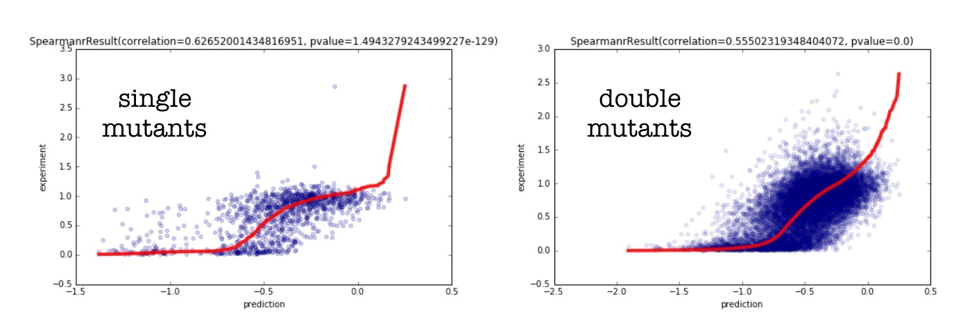
The red line denotes perfect rank correlation (spearman). The blue dots are the actual predictions vs. the experimental data. I can compare the performance of our model for both single and double mutants with that of Hopf. et al. In the table below, I show the spearman correlations between the experimental data, and that predicted by our method (approach 3), and compare it to the predictions done by the epistatic model (as well as the baseline independent model). I use the PABP yeast dataset[4] because it has both single and double mutant data.

The results I report here are without sequence reweighting. My references correct for oversampling (because MSA generates clusters of sequences), by dividing the weight of each sequence within a neighborhood by the size of its neighborhood. My experience suggests that while tuning the reweighting parameter \(\theta\) does improve the predictions for each dataset, picking a pre-determined \(\theta\) such that \(0<\theta\leq 0.2\) across all datasets doesn’t consistently improve our predictions across datasets and on occasion deteriorates our results. The reader is welcome to use the reweighting logic provided in the notebook to attempt this by themselves.

Method	Singles	Doubles
Independent	0.42	0.49
Epistatic (Hopf et al.)	0.59	0.52
VAE	0.63	0.56

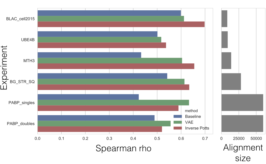
I also run the same process on 5 other available datasets. Below I show the comparison between the VAE’s performance and that of the EVmutation (Hopf et al.). As it can be seen, our method mostly outperforms the independent model, meaning we are capturing higher-order interactions in the sequence. However, it also appears that our model occasionally misses out on learning some pairwise interactions. Note that the \(P\) matrix in this comparison is slightly more complicated (see notebook for details).

Under the hood of the VAE

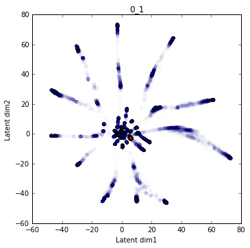
One particularly appealing aspect of the VAE is that it performs a non-linear compression of the data into a set of latent variables. What I hope to learn is whether this compression (encoding) scheme learned by the network can provide biological insight. In particular whether walking in the lower dimensional manifold that the network projects onto includes biologically relevant (and interpretable) features.

The training data (as projected in the latent domain) are presented in blue. The wildtype is indicated by a larger red dot.

There is more information to be extracted from the latent space. I redraw this structure, but color the background by computing the \(\mathbb{P}(\sigma_{wt})\) at each location using the \(H_{wt}\) as input and \(P\) as the PWM induced by that point in the latent space. White areas are where wildtype occurs with the same probability as it’s own coordinate in the latent space. Red means that wildtype is less favored in those locations, and blue means it is more favored. To better understand the basis of this structure, I have now also color coded the training data using k-means clustering.

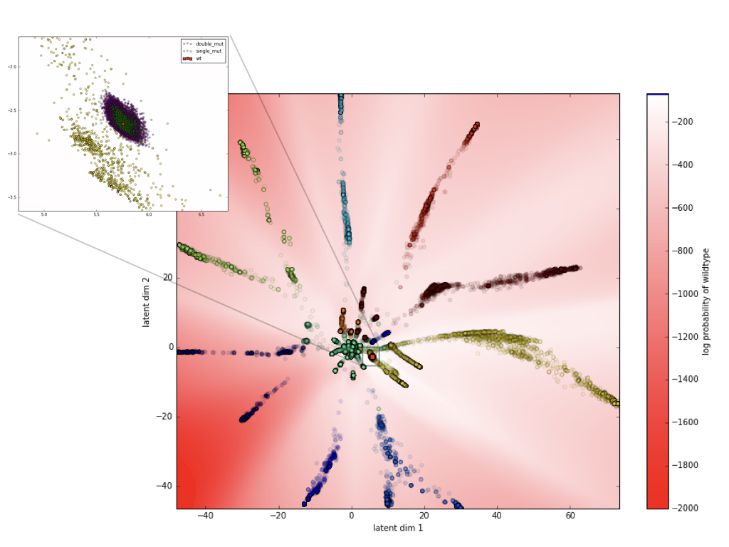
It is apparent that the clusters/branches in the latent dimension correspond to the min-distance clusters. In the zoomed in version near the wildtype (red dot), we can see the scatter of single (green) and double mutants (purple) where we have experimental data available. As it is clear, we only get to test the model on a very small region of the latent space. Ideally, our experimental data would also have sequences that are located in other parts of the latent space.

To get a better sense of what is occuring in the sequence space along the axis of maximum variance (in the neighborhood of the sequence of interest) I use PCA to compute the principal eigenvector using only the test data in the latent space (compressing the entire training data to one dimension is more lossy). I then walk along this axis in the latent space, this is presented in the animation below.

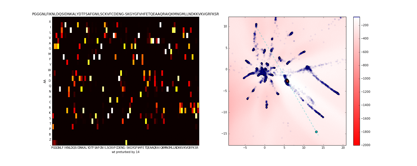
Walking in the latent dimension results in a variety of sequences. On the left panel, I show the distribution of sequences induced by the point corresponding to the cyan point in the latent space (on the right panel). The most likely sequence is written atop the left panel.

While these are interesting to observe, it remains unclear what we can learn from the structure of the latent space and the distributions that were learned for sequeneces in different coordinates of this space.

In the following segment, I touch on this, as well as other areas of this approach where I think suggestions by people with more experience in deep learning would be helpful.

Questions and areas for potential improvement

1- Hyper parameter optimization: While I have done some hyperparameter optimization (number of layers, regularization, dropout layers, number of hidden units) by random checking, I am not sure if there are obvious improvements that I am missing out on. ADAM is fairly robust to these changes, however, SGD, which presumably could find better optima, is rather sensitive and blows up quickly. I have not achieved better results with SGD compared to ADAM.

2-Network types: I have experimented with a simple convolutional architecture, as well as recurrent layers in my setup, none of which come close to the performance of the dense layers. In principle I expect the recurrent layers to learn useful information about the protein, but this has not materialized. What are some sensible architectures to test?

3-Interpretation of results: I have provided some interpretations for what the network outputs, and explored the latent space. However, it is clear that there is more lessons to be learned from the latent and hidden layers. What should I be looking for?

4-Long training: A lot of my runs, even on machines with large memory, result in memory errors mid training. I also get loss overflows (nan valued loss), when I use SGD with momentum (if I don’t clip the gradients aggressively). My guess is that this can be improved by hyperparameter tuning/regularization/constraining the network but how to correctly approach this is unclear to me.

Conclusion

This post serves as a proof of concept to demonstrate the ability of VAEs in capturing correlations in protein sequences. Interestingly, it works comparably to the “state of the art” methods that are based on Potts models. I am not the only one who has noticed this, and as mentioned before, Debora Marks’ lab has been working on a similar idea independently. In fact John Ingraham and Debora Marks have also written a nice paper on a variational inference as applicable to protein structure prediction[5]. However, I think that we are not currently using the full power of the model in practice. I hope that this post can help me and other interested researchers to improve on these results. Suggestions, ideas, and comments are welcome.

References

[1]: Ekeberg, Magnus, et al. “Improved contact prediction in proteins: using pseudolikelihoods to infer Potts models.” Physical Review E 87.1 (2013): 012707.

[2]: Hopf, Thomas A., et al. “Mutation effects predicted from sequence co-variation.” Nature Biotechnology (2017).

[3]: Kingma, Diederik P., and Max Welling. “Auto-encoding variational bayes.” arXiv preprint arXiv:1312.6114 (2013).

[4]: Melamed, Daniel, et al. “Deep mutational scanning of an RRM domain of the Saccharomyces cerevisiae poly (A)-binding protein.” Rna 19.11 (2013): 1537-1551.

[5]: Ingraham, John, and Debora Marks. “Variational Inference for Sparse and Undirected Models.” ICML 2017